47 Measures of Central Tendency and Variability

Central Tendency

The central tendency of a distribution is its middle—the point around which the scores in the distribution tend to cluster. (Another term for central tendency is average.) Looking back at Figure 9.1, for example, we can see that the self-esteem scores tend to cluster around the values of 20 to 22. Here we will consider the three most common measures of central tendency: the mean, the median, and the mode.

The mean of a distribution (symbolized M) is the sum of the scores divided by the number of scores. It is an average. As a formula, it looks like this:

M=ΣX/N

In this formula, the symbol Σ (the Greek letter sigma) is the summation sign and means to sum across the values of the variable X. N represents the number of scores. The mean is by far the most common measure of central tendency, and there are some good reasons for this. It usually provides a good indication of the central tendency of a distribution, and it is easily understood by most people. In addition, the mean has statistical properties that make it especially useful in doing inferential statistics.

An alternative to the mean is the median. The median is the middle score in the sense that half the scores in the distribution are less than it and half are greater than it. The simplest way to find the median is to organize the scores from lowest to highest and locate the score in the middle. Consider, for example, the following set of seven scores:

8 4 12 14 3 2 3

To find the median, simply rearrange the scores from lowest to highest and locate the one in the middle.

2 3 3 4 8 12 14

In this case, the median is 4 because there are three scores lower than 4 and three scores higher than 4. When there is an even number of scores, there are two scores in the middle of the distribution, in which case the median is the value halfway between them. For example, if we were to add a score of 15 to the preceding data set, there would be two scores (both 4 and 8) in the middle of the distribution, and the median would be halfway between them (6).

One final measure of central tendency is the mode. The mode is the most frequent score in a distribution. In the self-esteem distribution presented in Table 9.1 and Figure 9.1, for example, the mode is 22. More students had that score than any other. The mode is the only measure of central tendency that can also be used for categorical variables.

In a distribution that is both unimodal and symmetrical, the mean, median, and mode will be very close to each other at the peak of the distribution. In a bimodal or asymmetrical distribution, the mean, median, and mode can be quite different. In a bimodal distribution, the mean and median will tend to be between the peaks, while the mode will be at the tallest peak. In a skewed distribution, the mean will differ from the median in the direction of the skew (i.e., the direction of the longer tail). For highly skewed distributions, the mean can be pulled so far in the direction of the skew that it is no longer a good measure of the central tendency of that distribution. Imagine, for example, a set of four simple reaction times of 200, 250, 280, and 250 milliseconds (ms). The mean is 245 ms. But the addition of one more score of 5,000 ms—perhaps because the participant was not paying attention—would raise the mean to 1,445 ms. Not only is this measure of central tendency greater than 80% of the scores in the distribution, but it also does not seem to represent the behavior of anyone in the distribution very well. This is why researchers often prefer the median for highly skewed distributions (such as distributions of reaction times).

Keep in mind, though, that you are not required to choose a single measure of central tendency in analyzing your data. Each one provides slightly different information, and all of them can be useful.

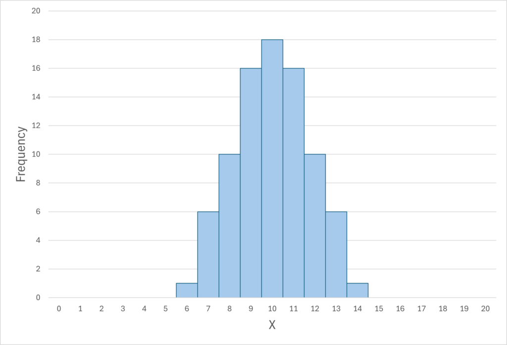
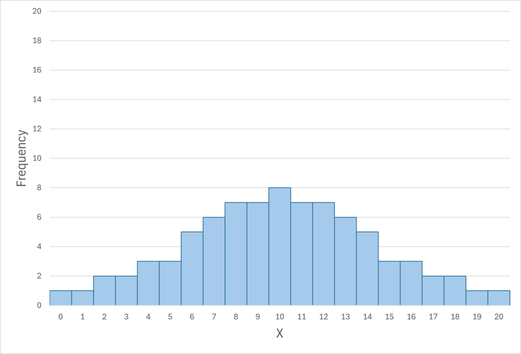
Measures of Variability The variability of a distribution is the extent to which the scores vary around their central tendency. Consider the two distributions in Figure 9.4, both of which have the same central tendency. The mean, median, and mode of each distribution are 10. Notice, however, that the two distributions differ in terms of their variability. The top one has relatively low variability, with all the scores relatively close to the center. The bottom one has relatively high variability, with the scores are spread across a much greater range.

One simple measure of variability is the range, which is simply the difference between the highest and lowest scores in the distribution. The range of the self-esteem scores in Table 12.1, for example, is the difference between the highest score (24) and the lowest score (15). That is, the range is 24 − 15 = 9. Although the range is easy to compute and understand, it can be misleading when there are outliers. Imagine, for example, an exam on which all the students scored between 90 and 100. It has a range of 10. But if there was a single student who scored 20, the range would increase to 80—giving the impression that the scores were quite variable when in fact only one student differed substantially from the rest.

By far the most common measure of variability is the standard deviation. The standard deviation of a distribution is the average distance between the scores and the mean. For example, the standard deviations of the distributions in Figure 9.4 are 1.69 for the top distribution and 4.30 for the bottom one. That is, while the scores in the top distribution differ from the mean by about 1.69 units on average, the scores in the bottom distribution differ from the mean by about 4.30 units on average.

Computing the standard deviation involves a slight complication. Specifically, it involves finding the difference between each score and the mean, squaring each difference, finding the mean of these squared differences, and finally finding the square root of that mean. We do not need to go into the details of how to computer it here, but rather what it means and how to interpret it.